CorWav IDL Library documentation

3. Setting up your local copy of CorWav.

You can download your local copy of CorWav from here, or by running the following in your command line terminal (assuming you have git installed):


$> git clone https://github.com/kkozarev/coronalwaves corwav

This will download a copy of the code into the local folder 'corwav'.

After this, there are several steps to take in order to ensure you can access the procedures and run them properly. First, you need to add some global variables to your linux/unix-like environment. Luckily, there's a script that can do that for you. Open the file set_paths.sh in gen/ directory of the code folder - you should see several variables like this near the top:


#set CORWAV to the directory where analyzed events will be stored
CORWAV="/Volumes/Backscratch/Users/kkozarev/corwav/"
#set CORWAV_DATA to the directory where the local copy of data will live
CORWAV_DATA="/Volumes/Itch/Users/kkozarev/corwav/"
#set CORWAV_TRUNK to the directory of the CorWav code (or local copy of the repository)
CORWAV_TRUNK="${HOME}/git/corwav/"
#set CORWAV_WEB to directory where the web database page is.
CORWAV_WEB="/var/www/personal/kkozarev/public_html/"
#If you want to back up the CorWav-analyzed events, set this variable too
CORWAV_DATA_BACKUP="/Volumes/Itch/Users/kkozarev/corwav/backup/"
#This can be used to set a cronjob in crontab, similar to this command:
10 00 * * * rsync -rvg --progress $CORWAV_DATA"events/" $CORWAV_DATA_BACKUP"events/"

Edit these to point to the code location (CORWAV_TRUNK), archived local data (CORWAV_DATA), the directory where analyzed data will live (CORWAV), and (optionally) the web database directory (CORWAV_WEB). Save and execute the script.

Top

4. Creating and loading an event.

An 'event' is a structure containing the necessary information that CorWav tools use to load and process coronal wave and related data, for a given solar eruption event. This information is instrument-independent. CorWav provides a human-readable, easy to use JSON format for loading event data into IDL. Here is an example of the input format for a single event:


{
"label": "110511_01",
"coordX": 785,
"coordY": 399,
"st": "2011/05/11 02:10:00",
"et": "2011/05/11 02:40:00",
"aiafov": [1024,2048],
"flareclass": "B8.1",
"typeII": true,
"loop": true,
"filament": true,
"comment": "Huge shock wave originates inside the limb, with clear lateral expansion.",
"web": false,
"rstn_lookup": "http://www.ips.gov.au/Category/World%20Data%20Centre/.../20110511spectrograph.gif",
"callisto_lookup": "",
"nrh_lookup": ""
}

The JSON format has elements (such as "label"), which have certain values (such as "110511_01"), assigned with the ':' character. The elements are separated by commas. Text values must be surrounded in quotation marks, unlike numbers. The format also accepts an array of values (such as "aiafov": [1024,2048]), or boolean values (such as "filament": true). Every instance of the structure format is surrounded by curly brackets. White space is unimportant for the JSON format, but it is very important for readable code.

Let's look at the elements in the event structure. The first one,


 {"label": "110511_01"}

is the unique label of the event. Its format is YYMMDD_NN, where YYMMDD is the date, and NN is the consecutive number of this event in the database for that date. Thus, "110511_01" is the first event of 11 May, 2011 in the event database. The event label is very important, since it is used to uniquely identify an event, along with all its information.


{
"coordX": 785,
"coordY": 399,
"st": "2011/05/11 02:10:00",
"et": "2011/05/11 02:40:00"
}

The next few elements specify the time and space position of the event. The first two, "coordX" and "coordY", give the coordinates, in arcseconds, of the origin of the eruption on the solar disk (these can be obtained most easily from Heliospheric Event Knowledgebase (HEK), although they are not always correct). These coordinates are used to determine the position of the event on AIA images and to automatically cut a subregion around it, together with the "aiafov" element (see below). "st" and "et" give the starting and ending times for the event. They are used to automatically fetch only the necessary data files for analysis. Note the particular datetime format, which is required for CorWav to parse the information properly.


{ 
 "aiafov": [1024,2048],
 "flareclass": "B8.1",
 "typeII": true,
 "loop": true,
 "filament": true
}

The "aiafov" element holds the X- and Y-sizes (in pixels) for the field of view to cut out from the 4096-by-4096 pixels of the original AIA data (Using the entire image is rarely necessary). The "flareclass" element holds the X-ray class of the flare (if there isn't one, leave a blank string). The best place to search for the class of a flare is Solar Monitor, or HEK. The next three elements take boolean values 'true' or 'false', depending on whether there was metric radio type II emission, expanding loops, or filaments.


{ 
"comment": "Huge shock wave originates inside the limb, with clear lateral expansion.",
"web": false,
"rstn_lookup": "http://www.ips.gov.au/Category/World%20Data%20Centre/.../20110804spectrograph.gif",
"callisto_lookup": "",
"nrh_lookup": ""
}

The element "comment" holds a free-form comment on the appearance and any interesting features of the particular event, by (ideally) the person who submits it. The "web" element is a tag specifying whether the event is ready to post on a website. The last three elments hold the urls or file names of quicklook plots of metric radio emission during the event, from three different networks of solar radio observatories. If no quicklook plots are available, this field should be left a blank string.

All the event entries your local CorWav copy. CorWav knows using the load_events_info() function

 IDL> event=load_events_in IDL> help,event EVENT           STRUCT

The result

 IDL> help,event,/st ** Structure <4827008>, LABEL ST ET COORDX          INT            785 COORDY          INT            399 AIAFOV          INT       Array[2] HEMISPHERE      STRING    'W' DATE            STRING    '20110511' ARLON           FLOAT ARLAT           FLOAT GEOMCORFACTOR   FLOAT FLARECLASS      STRING    'B8.1' TYPEII          INT              1 LOOP            INT              1 FILAMENT        INT              1 COMMENT AIA_DATAPATH NRH_DATAPATH RHESSI_DATAPATH STRING RSTN_DATAPATH CALLISTO_DATAPATH

RSTN_LOOKUP CALLISTO_LOOKUP STRING    '' NRH_LOOKUP      STRING    '' EUVI_DATAPATH   STRING SWAP_DATAPATH   STRING PFSS_DATAPATH   STRING SAVEPATH WEBPATH MOVIEPATH RADIOPATH NRHPATH RSTNPATH CALLISTOPATH ANNULUSPATH PFSSPATH SWAPPATH IONIZATIONPATH  STRING ASCHDEMPATH WEBERPATH PARTICLESPATH   STRING EUVIPATH DEMPATH PNGPATH YAFTAWAVEPATH   STRING KINEMATICSPATH  STRING AIA_SAVENAME ANNPLOT

As you can see, well - such as all the correction factor (more on that later). (individual structures) must be written/added to the file 'events.json' in the dat/ folder of to search for event information there. You can access the information you entered, and more, for a single event, by and specifying the event label: fo(label='110511_01') = -> Array[1] is a structure, let's see what's inside. 48 tags, length=672, data length=666, refs=1: STRING '110511_01' STRING '2011/05/11 02:10:00' STRING '2011/05/11 02:40:00' 64.0852 23.4466 1.11180 STRING 'Huge shock wave originates inside the limb, with clear lateral expansion.' STRING '/Volumes/Itch/Users/kkozarev/corwav/AIA_data/' STRING '/Volumes/Itch/Users/kkozarev/corwav/NRH_data/' '/Volumes/Itch/Users/kkozarev/corwav/RHESSI_data/' STRING '/Volumes/Itch/Users/kkozarev/corwav/RSTN_data/' STRING '/Volumes/Itch/Users/kkozarev/corwav/Callisto_data/' STRING 'http://www.ips.gov.au/Category/World%20Data%20Centre/Data%20Display%20and%20Downl'... '/Volumes/Itch/Users/kkozarev/corwav/EUVI_data/' '/Volumes/Itch/Users/kkozarev/corwav/SWAP_data/' '/Volumes/Itch/Users/kkozarev/corwav/PFSS_data/' STRING '/Volumes/Backscratch/Users/kkozarev/corwav/events/110511_01/' STRING '/var/www/personal/kkozarev/public_html/events/110511_01/' STRING '/Volumes/Backscratch/Users/kkozarev/corwav/events/110511_01/movies/' STRING '/Volumes/Backscratch/Users/kkozarev/corwav/events/110511_01/radio/' STRING '/Volumes/Backscratch/Users/kkozarev/corwav/events/110511_01/radio/NRH/' STRING '/Volumes/Backscratch/Users/kkozarev/corwav/events/110511_01/radio/RSTN/' STRING '/Volumes/Backscratch/Users/kkozarev/corwav/events/110511_01/radio/Callisto/' STRING '/Volumes/Backscratch/Users/kkozarev/corwav/events/110511_01/annulusplot/' STRING '/Volumes/Backscratch/Users/kkozarev/corwav/events/110511_01/pfss/' STRING '/Volumes/Backscratch/Users/kkozarev/corwav/events/110511_01/swap/' '/Volumes/Backscratch/Users/kkozarev/corwav/events/110511_01/ionization/' STRING '/Volumes/Backscratch/Users/kkozarev/corwav/events/110511_01/dem/aschwanden/' STRING '/Volumes/Backscratch/Users/kkozarev/corwav/events/110511_01/dem/weber/' '/Volumes/Backscratch/Users/kkozarev/corwav/events/110511_01/particles/' STRING '/Volumes/Backscratch/Users/kkozarev/corwav/events/110511_01/euvi/' STRING '/Volumes/Backscratch/Users/kkozarev/corwav/events/110511_01/dem/' STRING '/Volumes/Backscratch/Users/kkozarev/corwav/events/110511_01/png/' '/Volumes/Backscratch/Users/kkozarev/corwav/events/110511_01/yaftawave/' '/Volumes/Backscratch/Users/kkozarev/corwav/events/110511_01/kinematics/' STRING 'normalized_AIA_20110511_110511_01_' STRUCT -> Array[1] the structure contains not only the information we supplied through the JSON format, but a lot of additional information as necessary input and output directory paths, correction factors, active region coordinates in degrees, and a geometric You can load all the event information at once, by running load_events_info() with no arguments:


IDL> events=load_events_info()
IDL> help,event
EVENTS           STRUCT    = ->  Array[27]

Let's go back to event '110511_01'. Once you have its event structure loaded, you can pass it as an argument to many CorWav tools. Next, you will see how to load some AIA data and make movies from it. Oh, and by the way, calling load_events_info for the first time for an event causes it to create the event's directory tree in the CORWAV directory, so no need to worry about that.

Top

5. Loading AIA data. Processing AIA data, making images and movies.

To load and preprocess (prep) AIA data, use the aia_load_data procedure. It loads the AIA data from the local or remote archive and preprocesses/calibrates it.


IDL> event=load_events_info(label='110511_01')
IDL> aia_load_data,event.st,event.et,'193',/remove_aec,index=index,data=data

Running the above will return to the user the descriptive information (the index) and the data itself in a three-dimensional array(n_times,nx,ny).If you wanted just the sub-region with the eruption, run with the subindex and subdata keywords, like this:


IDL> aia_load_data,event.st,event.et,'193',/remove_aec,subindex=subindex,subdata=subdata

In addition, the '/force' keyword tells the procedure to overwrite whatever data there is already saved. aia_load_data has many other options, which you can find by opening the file $CORWAV_TRUNK/aia/aia_load_data.pro. For example, an important option is to not include files with much shorter exposure that are often created during flares, by supplying the /remove_aec keyword.

In general, most of the procedures have additional keywords, described in the individual procedure files in the $CORWAV_TRUNK folder.

Once aia_load_data has executed successfully, you can make image files from the data, like this (1024x2048 px) base difference image:

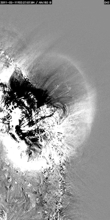
The command for making such images for all time steps of a specific event ('110511_01' in our case) and specific wavelength channel (193) is:


IDL> aia_make_images,event,'193',/base

You can do this for multiple types of images, and multiple wavelength channels, like this:


IDL> for w=0,n_elements(wav)-1 do aia_make_images,event,wav[w],/raw,/base,/run

The '/raw','/base','/run' keywords tell the procedure to make image files from the raw data (with an inverted color table to highlight the faint waves), base difference images (subtracting the first image from all consequent ones), or running difference images (subtracting the preceding image from the next one). Running the above will create PNG files in $CORWAV/events/110511_01/png/[type]/[wav]/,type being one of raw/base/run.

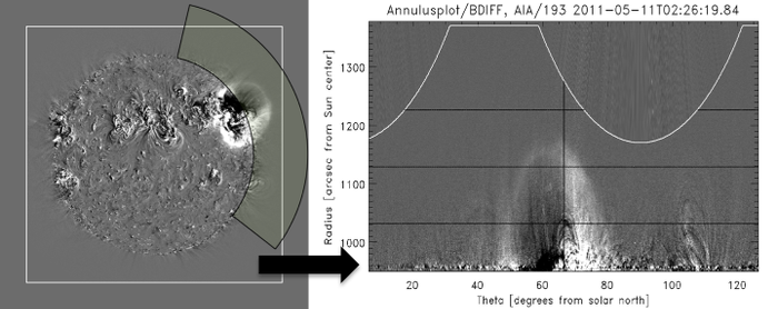
You can also create annulus data. Those are images created by deprojecting, or 'stretching' a part (annulus) of the solar image onto a rectangular canvas, where the X-axis is angular distance from solar north along the limb, and the Y-axis is radial distance from Sun-center. The figure below shows the AIA field of view (white square), the data in original form with the overlaid annulus to be deprojected (left), and the resulting deprojected annulus:

To convert the original data to annulus data, first run the following:


IDL> cashew_aia_annulus_create,event,wav='193',/base,/force,/remove_aec

This will create an annulus datacube, and place it (together with some other important variables) into a .sav file into the folder $CORWAV/events/110511_01/annulusplot/. To run this for all wavelengths and data types (raw,base,run), run:


IDL> for w=0,n_elements(wav)-1 do cashew_aia_annulus_create,event,wav=wav[w],/remove_aec

To make images of the annulus data, run the aia_annulus_plot command:


IDL> for w=0,n_elements(wav)-1 do aia_annulus_plot,event,/raw,/base,/run,wav=wav[w]

Running the above will create PNG files in $CORWAV/events/110511_01/annulusplot/[type]/[wav]/, type being one of araw/abase/arun. This procedure has other functionality, such as specifying the latitudinal (thrange keyword) and radial (rrange keyword) ranges for the plots, as well as overplotting the lines along which radial and latitudinal measurements will be taken, for context (add the /lines keyword).

Now that we have created some images of both the original and the annulus-deprojected data, we can create time lapse movies from them, like so:


IDL> aia_make_movies, event, movie_type='run', wav='193'

We just made a running difference .mp4 movie for this event. It will be stored in $CORWAV/events/110511_01/movies/.

If you want to make multiple types of movies for multiple wavelengths - for example, movies of all types of images we created above - you can do something like the following:


IDL> movie_types=['araw','abase','arun','raw','base','run']
IDL> for w=0,n_elements(wav)-1 do $
	    for mt=0,n_elements(movie_types)-1 do $
		   aia_make_movies, event, movie_type=movie_types[mt], wav=wav[w]

This created six different movies, and again put them in the folder $CORWAV/events/110511_01/movies/. The '$' sign in the IDL code above just allows to break the line without IDL complaining. If the movies exist already, you may have to add the /force keyword to the command, in order to write over the old ones.

Top

6. Measuring EUV wave kinematics.

There are different ways to measure how fast the wave is moving and how much it is accelerating/decelerating as a function of time. The usual way is to record the pixel values along a single radial line passing through the wave front and through the center of the Sun, as a function of time. This way, we can measure the evolution of the apparent edge (front) of the wave in the radial direction. The annulus images allow us to do that, but they also allow us to easily measure the lateral motion of the wave at different heights above the solar limb, which can give us information about the local plasma properties, as well as the eruptive feature that drives the wave. This is because we can simply measure the feature move along a row of pixels in the annulus images, which represent a constant height above the solar surface. The CorWav library allows the user to measure the radial and lateral motions along specific directions (black vertical and horizontal lines), shown in this automatically generated plot (white line denotes the edge of data):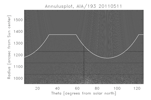 AIA annulus image with image edges and kinematics measurement "slits" width=0.1

We will start with the radial measurements. The procedure to use is 'aia_annulus_analyze_radial':


aia_annulus_analyze_radial,event,wave='193'

This will automatically measure the temporal and radial extent of the measurement. It will create a J-map - a plot which stacks the pixel values along the particular radial direction we've chosen for consecutive times next to each other, thus making a plot like the one below. Again, this could be done for multiple AIA channels, and the radial range manually constrained, like so:


IDL> rrange=[1.1,1.37] ;The radial range of the annulus to use (Rs)
IDL> for w=0,n_elements(wav)-1 do aia_annulus_analyze_radial,event,wave=wav[w],rrange=rrange,/constrain

The rrange keyword contains the radial range of the annulus image to use, in solar radii. The 'constrain' keyword tells the procedure to constrain the wave front to behave physically, allowing radial speeds between 10 and 1500 km/s. The procedure is interactive, and will produce a plot like this: 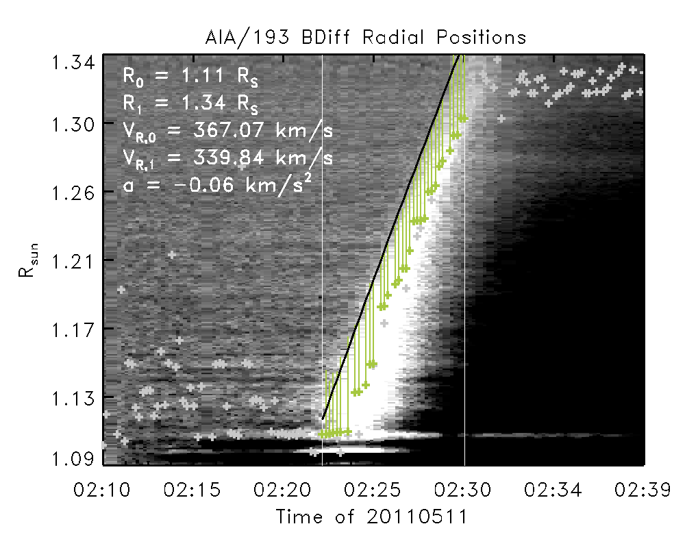AIA annulus base difference image
It will be automatically saved as a .png file in the CORWAV/events/110511_01/annulusplot/ folder, together with all the variables in a .sav file. The black line is a fit to the front of the wave, with the fit parameters written on the plot. The white vertical lines are the start and end times for fitting the wave front - these must be supplied by the user of the procedure (currently). The underlying greyscale plot was made by taking one column of the annulus image (centered on the AR position) at every time step, and stacking it next to the others. This produces a time-height plot, also known as a 'J-map'.

Top

7. Running the DEM, PFSS+CSGS models.

To be able to say more about the likely plasma and magnetic conditions, we need to apply several models, which use as inputs AIA observations or parameters inferred from these observations. These models are the essence of the analysis, and CorWav provides interfaces to them.

7.1 DEM

The first one is Differential Emission Measure analysis, which allows to use the multi-wavelength observations of AIA to calculate the amount of emitting material along the observed line of sight - a proxy for the coronal density. Currently, CorWav provides an interface to the DEM model of Aschwanden et al., 2013. This model fits a single Gaussian profile to the EUV emission as a function of temperature, and provides, for every pixel and time step, a value of the Emission Measure (EM) and the temperature of maximum emission (Tmax). This is how the model is run (including the /remove_aec keyword in order to remove any artefacts from flare exposure corrections):


IDL> aia_cfa_teem_run,event,/remove_aec

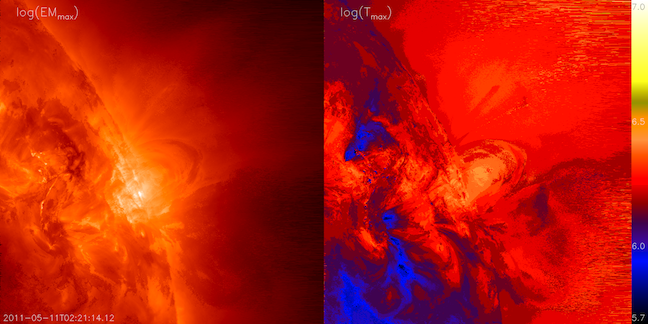
This will analyze data for every timestep and the specified field of view, and create a map of EM and Tmax. The individual time maps will be stored in the CORWAV/events/110511_01/dem/aschwanden/ folder, in PNG and SAV files. Here is the result for a single snapshot of the 110511_01 event:

Next, the time series of EM and Tmax for particular regions around the EUV wave sheath can be extracted, assuming the wave kinematics measurements have been performed.

	
IDL> aia_dem_define_subrois,event
IDL> aia_aschdem_save_subrois,event

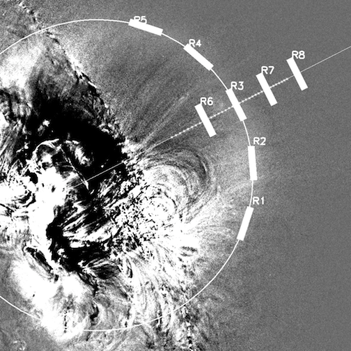
This procedure automatically positions 8 rectangular regions of interest (ROI) tangentially to the shock surface, four along the shock surface for the middle time step, and four along a radial direction outward from the eruption source, like in the following image. The results are saved in the CORWAV/events/110511_01/ionization/ folder. The aia_aschdem_save_subrois procedure extracts the DEM results at the previously defined ROIs.

The user can also choose to extract square ROIs interactively, using the aia_dem_define_subrois_manual procedure:

	
IDL> aia_dem_define_subrois_manual,event,numroi=8,roisize=10
IDL> aia_aschdem_save_subrois,event

where numroi is the number of ROIs to select, and roisize gives the square ROI size, in pixels.

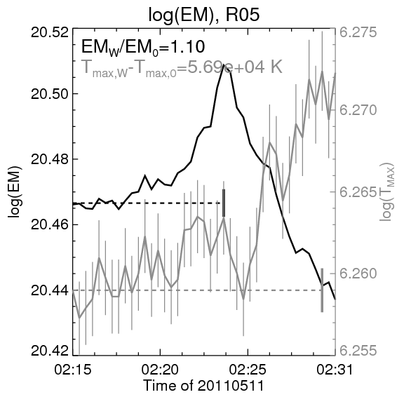
Once the DEM model has been run, and the ROIs have been selected, we can plot time series of EM and Tmax for them, using the aia_dem_analyze procedure:

	
IDL> trange='2011-05-11T'+['02:15:00','02:31:00']
IDL> aia_aschdem_analyze,event,trange=trange

Running this will produce individual PNG and SAV files for all selected regions in CORWAV/events/110511_01/dem/aschwanden/ with information on the time evolution of EM and Tmax. Here's a plot for one region for this particular event:

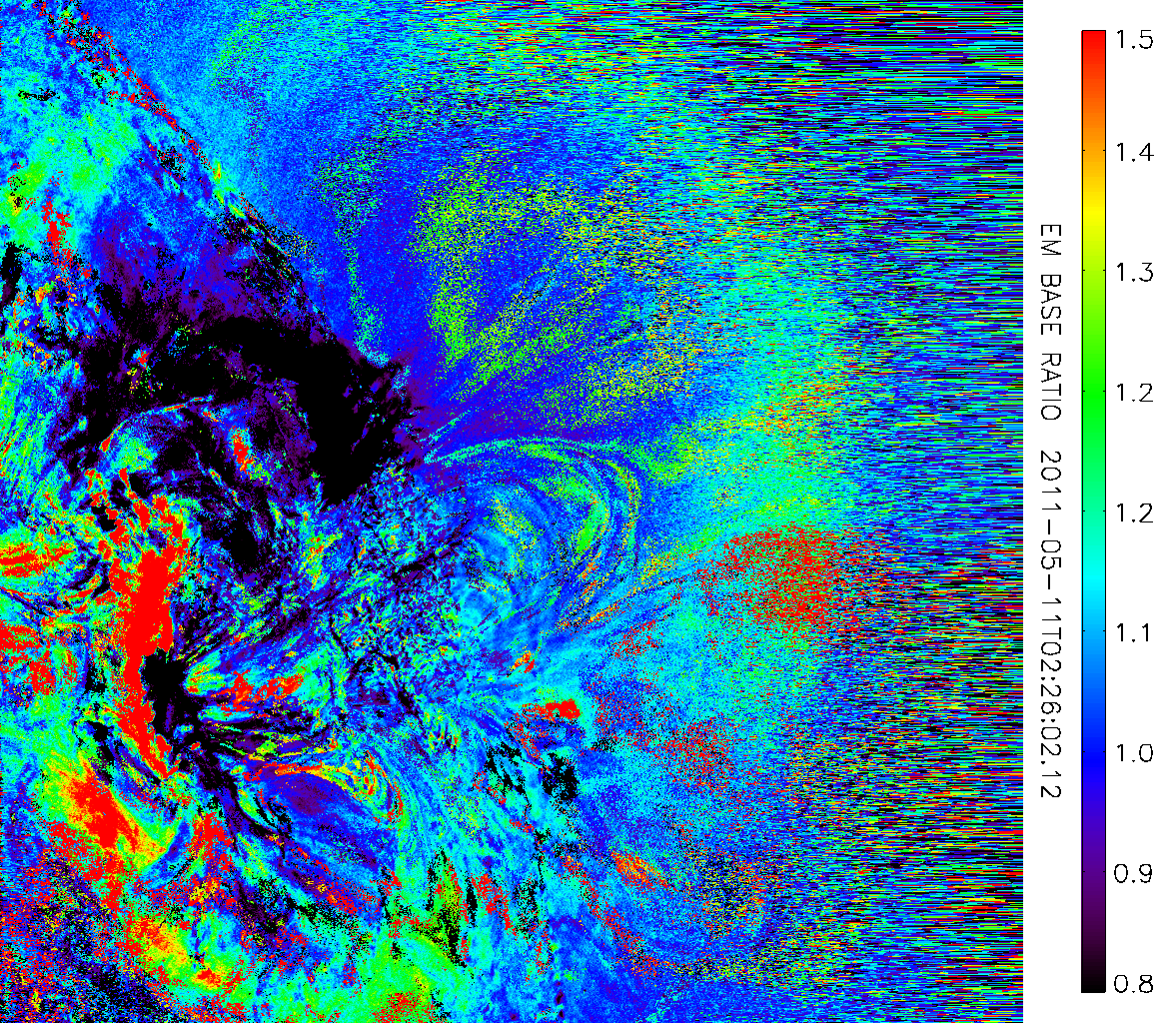
In addition, the user may create plots of the base emission measure base ratios (ratio of each EM image to the pre-event image) like the one below by running:

	
IDL> aia_aschdem_plot_em_ratios,event

7.2 PFSS+CSGS

To obtain information about how efficient the shock wave may be in accelerating particles to high energies, we combine a 3D static model of the coronal magnetic fields with a 3D evolving model of the shock surface. The magnetic field model (Schrijver and De Rosa, 2003) is known as a Potential Field Source Surface (PFSS) model, and is freely available as part of SolarSoft. It is driven by observations of photospheric line-of-sight magnetic fields over a full solar rotation, and produces extrapolations of that magnetic field in the corona out to ~2.5 solar radii. The CSGS model has been developed specifically for CorWav, and is part of this library. It uses the kinematic measurements for the wave radial edge positions to create a spheroidal surface, which represents the entire surface of the wave. Combining the two models allows the estimation of the time-dependent shock-to-field angle values and magnetic coronal connectivity for the shock event.

To apply the PFSS model, we first need to generate an instance of it for the nearest time to the event. This is done with the pfss_return_field procedure:

	
IDL> pfss_return_field,event.st,/save,path=event.pfsspath,event=event

The result is a large file, which will automatically be saved in CORWAV/events/110511_01/pfss/ folder. Next, run the pfss_shock_run_csgs procedure. It will create the CSGS model, and combine it with the PFSS model, to produce the positions at which the magnetic field lines cross the shock surface, and the crossing angle values. The results are saved again in the pfss/ folder.

	
IDL> pfss_shock_run_csgs,event

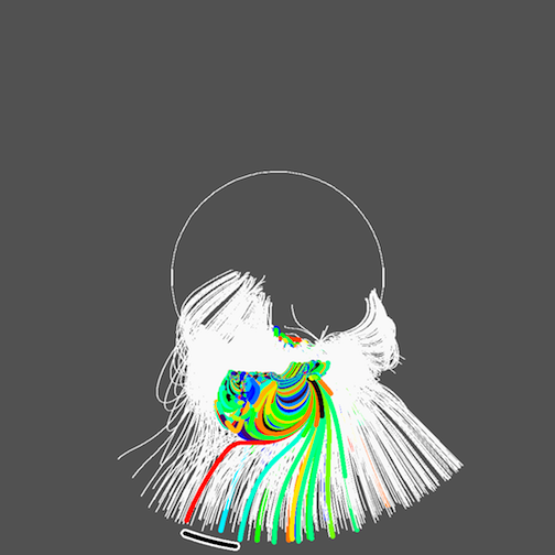
The images below illustrate the application of the PFSS+CSGS model. The loopy lines of represent the modeled coronal magnetic field lines near the time of the event. Orange lines are magnetically closed, blue ones are open. The black meshed surface is the CSGS model for that time step, and the green points represent the field line crossings. This plot was created by running

	
IDL> pfss_shock_plot_csgs,event,/png

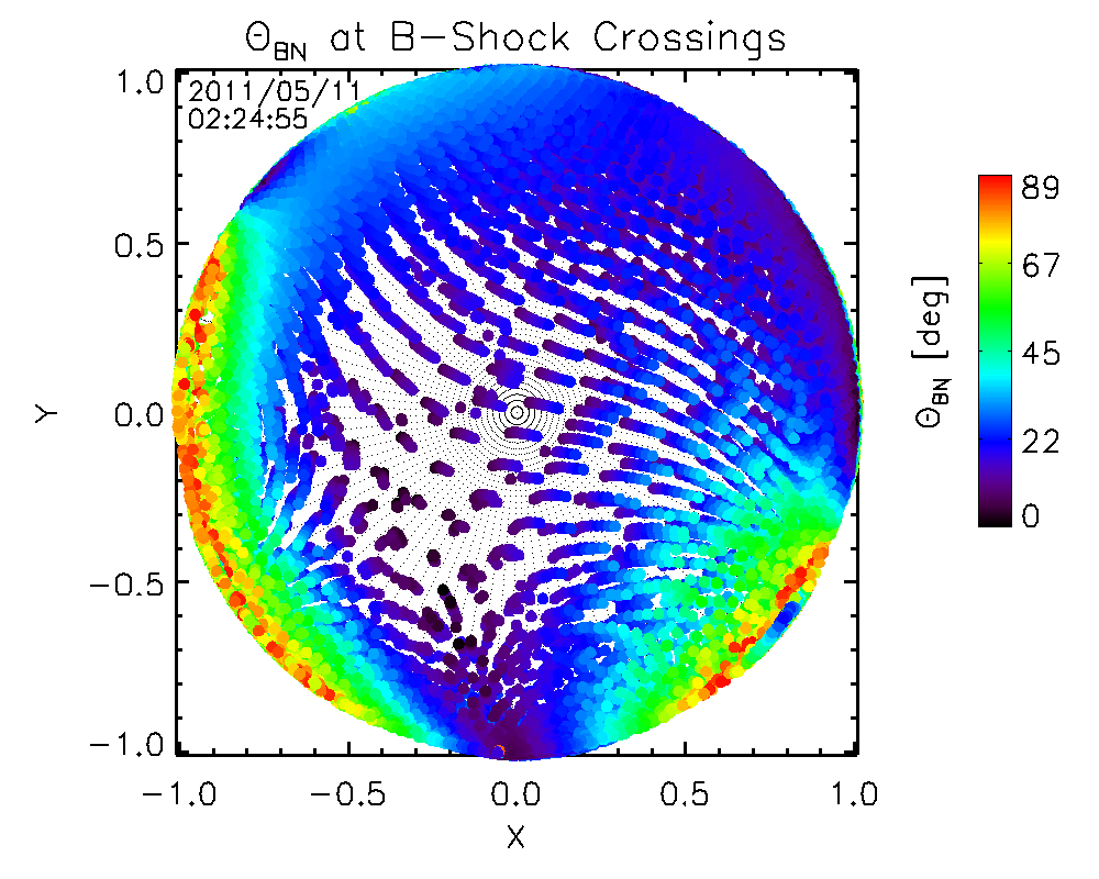
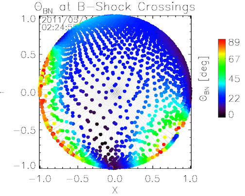
To plot the values of the shock-crossing angle (known as ThetaBN) for all time steps, run pfss_shock_plot_crossing_angles. It will produce one image for every time of the top-down view of the shock surface with the position of the shock crossings up to that time step (if you specify the /oplot keyword), and color-coded angle value (left image). Open field line crossings are open symbols. Without the /oplot keyword, the image will only contain the current crossings positions and angle values (right image).

	
IDL> pfss_shock_plot_crossing_angles,event(,/oplot)

You can obtain some statistics on the ThetaBN values over time and make a plot of them, by running

	
IDL> pfss_shock_plot_thetabn_stats,event

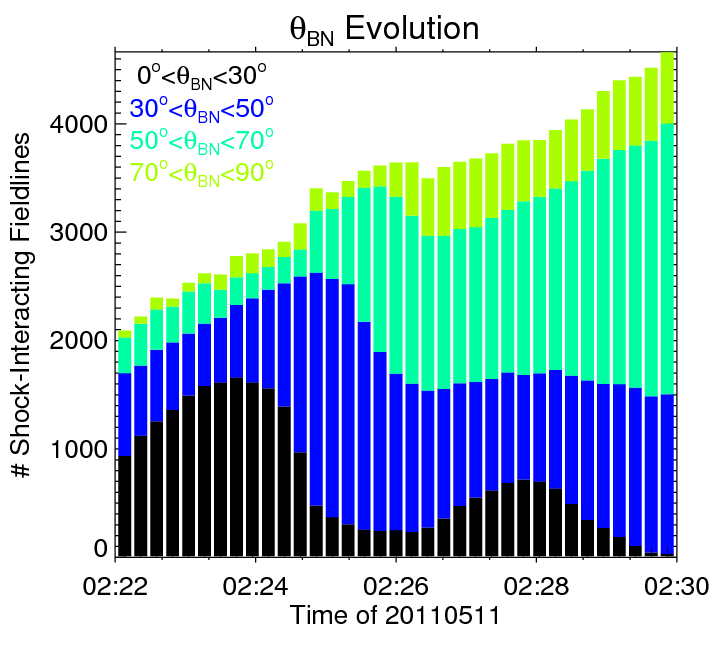
This procedure produces several statistical plots for the event: 1) one showing the crossing angles over time, 2) the same one augmented with plots of the open field lines crossed over time, and 3) a plot of the radial ranges of the open field crossings.

Finally, you can plot the coronal connectivity of the shock (all field lines that interact with the shock) for all time steps, using pfss_shock_plot_angular_influence. It will produce PFSS images with crossing field lines highlighted (orange for closed, light-blue for open), in a face-on view. The images can also be done in a top-down view, if we specify the /topview keyword:


IDL> pfss_shock_plot_angular_influence,event[,/topview]

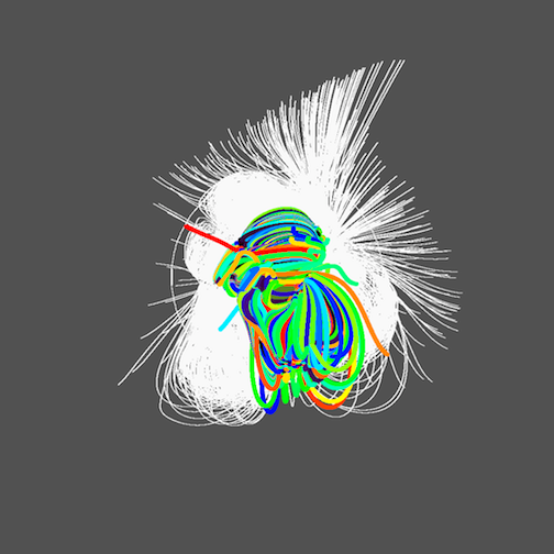
The top view has the advantage that it shows more readily the heliospheric connectivity, as well as the longitudinal range of magnetic field lines, which are nominally connected to near-Earth space (black arc), for solar wind speeds between 400 and 500 km/s.

All the plots shown in this section are generated automatically, and may be found in the /dem/aschwanden or /pfss/ folders of the respective event.

Top

CorWav IDL Library Documentation

Version 0.1.0.

Contents:

1. What is CorWav?

2. What tools does CorWav include?